
Rack Line Throughput Math: Cycle Time & Loading Density
More pieces on a rack do not automatically mean more saleable pieces per shift. Management-level rack-plating technicians must connect loading geometry, electrical demand, plating residence time, transfer capacity, and first-pass yield. Otherwise, an apparent capacity improvement becomes thin recesses, overloaded contacts, or a queue at unloading.
1. Establish a bounded operating model
The worked model concerns nickel deposition on properly copper-plated zinc-alloy bag fittings. It is not a direct nickel-on-zinc recipe. Pretreatment, copper coverage, subsequent finishes, and customer acceptance requirements remain separate qualification gates.
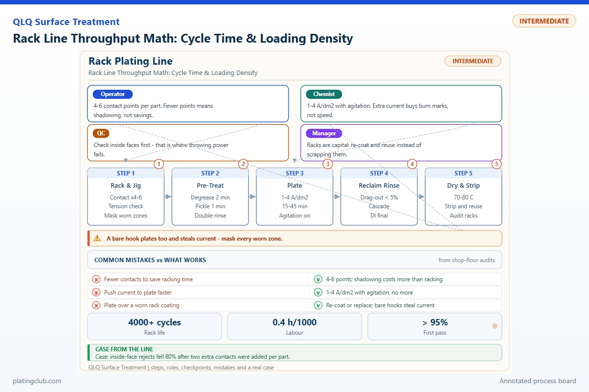
The QLQ knowledge note 018 — Rack Plating lists 50–200 pieces per rack, 1–5 A/dm2, 5–30 minutes plating time, copper layers of 3–8 µm, and nickel layers of 5–15 µm. These are contextual reference ranges, not guaranteed equipment capacity. The worked assumptions below use 120 pieces, 0.05 dm2 plated area per piece, and a 20-minute nickel dwell.
Start with a timed route sheet: loading, cleaning, activation, copper, rinses, nickel, any final finish, drying, unloading, and inspection. Record powered deposition separately from immersion and transfer. Identify usable rack positions, shared hoists, rectifier allocation, loading labor, and buffer locations. A machine model number alone cannot establish the dispatch interval.
2. Separate residence time from dispatch interval
Residence time is how long one rack spends in a stage. Dispatch interval is the spacing between successive rack releases. For a stage with m equivalent positions, the optimistic interval is Tstage = residence time / m. The actual schedule must include clearance, transfer conflicts, drainage, and loading availability.
Four independent nickel positions with a 20-minute dwell imply a five-minute theoretical interval. If the validated scheduler needs 30 seconds of clearance per release, use a provisional 5.5-minute interval, not five. This allowance is an example; derive yours from event logs.
Gross output = 60N / T, where N is pieces per rack and T is dispatch interval in minutes. Accepted output = gross output × availability × first-pass yield. With 120 pieces, T = 5.5 minutes, availability = 0.90, and yield = 0.97, the result is approximately 1,143 accepted pieces per scheduled hour.
That is a hypothetical steady-state calculation, not a QLQ production promise. Shift output also depends on startup filling and end-of-shift drainage. Do not multiply by eight hours when only six hours contain completed rack releases. Do not apply availability twice if your measured average interval already includes downtime.
For loading, two workers each taking eight minutes per rack provide an average four-minute capacity interval only if they work independently. Include unloading and inspection labor before accepting that figure. For a 70-minute end-to-end route at T = 5.5 minutes, steady-state work in process is approximately 70/5.5 = 12.7 racks; spare racks and maintenance buffers are additional.
3. Working Data & Formula Notes: area, current, and thickness
A = Na + Arack; I = jA. A is total electrically exposed cathode area in dm2, a is plated area per piece, and j is average cathode current density. Include exposed rack metal; exclude insulated metal. For clarity, the calculations below neglect exposed rack area, which must be measured before implementation.
At 120 × 0.05 = 6 dm2 and j = 2.5 A/dm2, demand is 15 A. At 160 pieces, area becomes 8 dm2 and demand becomes 20 A. Holding current at 15 A reduces average j to 1.875 A/dm2. Keeping current density constant may still worsen local distribution because neighboring parts shield each other.
For nickel, Faraday's law gives d ≈ 0.205 ηjt, with d in µm, t in minutes, and current efficiency η as a fraction. The coefficient follows from nickel molar mass, divalent deposition, Faraday's constant, and nickel density. At assumed η = 0.95, j = 2.5, and t = 20, the calculated average is 9.74 µm. This predicts average metal deposition, not the minimum thickness inside a recess.
| Component | Range | Typical | Function | Replenishment |
|---|---|---|---|---|
| Nickel sulfate hexahydrate, NiSO4·6H2O | 240–300 g/L | 270 g/L | Principal nickel-ion source | Maintain soluble nickel anodes; correct verified analytical deficit and drag-out losses. |
| Nickel chloride hexahydrate, NiCl2·6H2O | 30–90 g/L | 60 g/L | Supports conductivity and anode dissolution | Analyze chloride; add measured salt corrections, accounting for other chloride inputs. |
| Boric acid, H3BO3 | 30–45 g/L | 40 g/L | Buffers conditions near the cathode | Analyze, dissolve through an approved procedure, mix, and recheck. |
| Deionized water | Balance | To final volume | Solvent and concentration control | Restore marked volume for evaporation before interpreting concentration trends. |
The base ranges come from the Nickel Institute Nickel Plating Handbook, which also gives 40–60 °C, pH 3.5–4.5, and 2–7 A/dm2 for Watts operation. Typical values here are selected within those ranges. This is a complete base electrolyte, not a complete proprietary bright-nickel system: brighteners and wetting agents require supplier-specific instructions.
For a verified salt deficit, addition in kg = deficit in g/L × working volume in L / 1,000, corrected for assay. Distinguish nickel-metal analysis from hydrated-salt concentration. Never dose nickel salts solely by ampere-hours: soluble anodes replace deposited metal, while drag-out and anode performance determine the net balance.
4. Controlled rack-density trial: calculations and required measurements
Evidence status: no measured density-comparison dataset was supplied or found in the consulted QLQ notes. This table is a calculated trial comparison, not experimental evidence. XRF minima, salt-spray results, and hardness remain unmeasured; do not convert these predictions into a test certificate.
| Batch / loading | Test condition | Calculated average Ni | Measured minimum Ni | Corrosion / hardness | Decision |
|---|---|---|---|---|---|
| A: 120 pieces; 6 dm2 | 15 A; 20 min powered dwell; 50 °C; pH 4.0; fixed rack orientation | 9.74 µm | Not measured | Not tested | Baseline candidate |
| B: 160 pieces; 8 dm2 | 15 A; 20 min; same bath and orientation; average j = 1.875 A/dm2 | 7.30 µm | Not measured | Not tested | Predicted average below illustrative 8 µm minimum |
| C: 160 pieces; 8 dm2 | 20 A; 20 min; same bath and orientation; average j = 2.5 A/dm2 | 9.74 µm | Not measured | Not tested | Requires local-thickness and thermal qualification |
Run at least three racks per condition as an initial engineering comparison. Keep substrate lot, copper underlayer, chemistry, anode layout, and transfer sequence constant. Rotate trial order to reduce time-of-day bias. Map top, middle, bottom, center, and edge positions; measure exposed and sheltered significant surfaces with a validated multilayer XRF program.
Use an illustrative minimum of 8 µm only if quality approves it for this trial. Report minimum, mean, spread, measurement uncertainty, rejects, and actual dispatch interval. Test corrosion on the complete customer-specified coating stack using an agreed method and acceptance criterion. Nickel thickness alone cannot establish salt-spray life; hardness also cannot be inferred from ampere-hours.
5. Trend bands and escalation thresholds
These are proposed internal limits for the worked model, not universal defect boundaries. Approve them against supplier instructions and qualification results. A warning prompts verification; a hold threshold prevents further dispatch until an authorized assessment.
| Parameter | Normal fluctuation band | Warning / danger threshold | Response |
|---|---|---|---|
| Nickel-bath pH | 3.8–4.2 around 4.0 | Warning outside band; hold below 3.5 or above 4.5 | Verify probe and sample temperature; authorize correction. |
| Bath temperature | 48–52 °C | Warning outside band; hold below 45 or above 55 °C | Check independent thermometer, heater, and circulation. |
| Average current density | 2.4–2.6 A/dm2 | Hold outside validated 2.0–3.0 window | Reconcile current with actual area and contact condition. |
| Powered nickel dwell | 19.8–20.2 min | Hold below 19.5 min; investigate above 20.5 min | Check current-on timestamps, not immersion alone. |
| 120-piece rack occupancy | 118–120 approved positions | Hold any unapproved position or count above 120 | Use a separate recipe for changed area or spacing. |
| Dispatch interval | 5.5–5.8 min under steady operation | Hold unvalidated acceleration below 5.5; investigate above 6.0 | Identify transfer conflicts and station starvation. |
| First-pass yield | 97–100% planning band | Investigate below 97%; management escalation below 95% | Contain relevant lots; classify defects by rack position. |
6. Two management decisions worked through
Scenario one: a dense rack exceeds the useful current envelope. Assume the validated continuous limit of the complete electrical path is 18 A. A 160-piece rack requires 20 A at the chosen density, so it is not an approved production setting. At constant 15 A, restoring the calculated 9.74 µm average requires 26.67 minutes. Four nickel positions plus the illustrative clearance then give T = 7.17 minutes. Gross output is about 1,340 pieces/hour, barely above the original 1,309, before any yield penalty. The remedy is a qualified geometry or electrical upgrade, not silently extending dwell.
Scenario two: loading becomes the bottleneck. Suppose two independent loaders need 12 minutes each for a complicated fitting: their effective capacity interval is six minutes. Improving nickel dispatch from 5.5 to five minutes cannot overcome that loading limit. Compare fixture access, staged part presentation, and dedicated unloading support. With 120 pieces, a six-minute interval, 90% availability, and 97% yield, accepted output is 1,048 pieces/hour. Revalidate the complete schedule after any labor change.
Both scenarios are transparent engineering examples, not claimed customer outcomes. Assign ownership across production, maintenance, bath control, and quality. Rank projects by incremental accepted output and cost per accepted piece, including rejects, chemicals, electricity, wastewater treatment, and labor.
7. Engineer Notes
- Measure plated area from drawings or validated geometry; attach the area revision and current setpoint to each rack recipe.
- Photograph the approved spacing and orientation. Block spare hooks that would allow operators to add unqualified pieces.
- Inspect contact springs and insulation before use. Measure loaded voltage drop and temperature against the qualified baseline; isolate power before servicing.
- Export one shift of hoist and rectifier timestamps. Separate blocked transfers, empty positions, current interruptions, and planned downtime.
- Change one density variable at a time. Quarantine trial racks until local thickness, adhesion, and required final-stack tests pass.
- Balance shared rectifier demand across simultaneous racks; verify the continuous duty limit of buses, contacts, and cables as well as the rectifier.
- Review daily accepted output with defect maps. Require signed approval before revising occupancy, dwell, or dispatch limits.
8. Shift Checks
| Shift stage | Check item | Frequency | Acceptance standard | Record |
|---|---|---|---|---|
| Before shift | Recipe, rack insulation, contacts, spacing | Every rack before loading | Approved map; intact insulation; no damaged contacts | Rack ID and operator signoff |
| Before shift | pH, temperature, bath volume, analytical status | Startup and after corrections | Approved bands; analysis current; circulation operating | Bath log and instrument ID |
| During shift | Occupancy, current, powered dwell | Every rack; automatic logging preferred | Match area-linked recipe and approved timing | Batch and rectifier event trace |
| During shift | Local thickness and appearance | First rack, hourly, and after change | Approved local minimum; no missing deposit, burning, or pinholes | XRF map, uncertainty, reject code |
| During shift | Dispatch, queues, contact heating | Hourly and on alarm | Validated schedule; thermal baseline not exceeded | Downtime reason and maintenance ticket |
| After shift | Output reconciliation and handover | Each shift | Accepted, rejected, held, and work-in-process counts reconcile | Shift report and signed containment handover |
9. FAQ: technician-to-AI troubleshooting prompts
These are suggested conversational prompts, not quotations attributed to documented customer correspondence.
AI, we added 40 pieces to each rack, but the center parts are thin. Should I increase current or time?
First recalculate area and check contacts, orientation, and shielding. Increasing current may burn edges without restoring sheltered thickness. Compare the three trial conditions above, then qualify a spacing change. Extend time only after confirming that distribution and the resulting line interval remain acceptable.
AI, our nickel dwell is 20 minutes. Why can the line release a rack every five minutes?
Parallel positions let several racks receive their full dwell simultaneously. Four equivalent positions give a theoretical five-minute spacing, not a five-minute plating time. Check shared electrical capacity, hoist conflicts, and transfer clearance before adopting that interval.
AI, production says output increased, but quality says we are losing money. Which KPI should I show management?
Show accepted pieces per scheduled hour alongside cost per accepted piece, minimum local thickness, and first-pass yield. Keep held parts out of accepted output. Separate capacity assumptions from measured results, and compare like-for-like product mixes before recommending investment.
10. What Would You Like to Solve?
Send your rack drawing, plated area, coating specification, rectifier allocation, station occupancy, timing log, and thickness map to [email protected]. These inputs support a defensible bottleneck review rather than a pieces-per-rack guess. See the integrated surface-treatment line support overview for equipment, chemistry, and process coordination.
Local source notes: QLQ Obsidian Vault, 02-Product Knowledge / IMA Company Knowledge / 018 — Rack Plating; 07-Surface Treatment / Rack and Barrel Plating; and 03-Equipment Knowledge / Rack and Barrel Plating Equipment. Source titles are translated into English. Public electrolyte reference is linked in Section 3. Calculations, proposed limits, and trial plans are explicitly distinguished from measured evidence.